Serving Tensorflow models with custom output signatures using TF Serving

tf

There are rather easy-to-follow and well-written tutorials to learn about serving tensorflow models for production using the Tensorflow Serving framework. These tutorials deal with machine learning models that typically return a single value following predict() or classify() calls. TF Serving requires some fine-tuning to properly serve machine learning models that can return multiple values like dictionaries. I only found scarce documentation to up-configure TF Serving to serve this type of models which can return dictionaries.

The purpose of this article is to explain some basic concepts of Tensorflow models and the Tensorflow Serving framework using a simple language, and give an hands-on introduction on serving models that can returns multiple output values.

Few Concepts for understanding Tensorflow Serving:

Model Signature:

Model Signature is a JSON-like serialized string (I think it is called Protocol Buffer in Googlosphere, I believe it is Google’s inhouse serialization tool) that informs an external agent on how to one could call a tensorflow model and what could one expect in return.

External agent here is the Tensorflow Serving framework which wraps tensorflow model artefacts, and obviously it has no idea on how to call these. Model signatures determine how this can be done. This is by the way not a Tensorflow specific concept.

Model Artefacts: Saved Models

Well initially you are writing a Python code using tensor objects as implemented by the Tensorflow mathematical library, representing ultimately a bunch of connected graphs and nodes. However, TF Serving is not going to execute your model represented as a Python code, it will call an abstraction of it. That is to say, it doesn’t require a Python backend interpreter.

This is what is called in TF a Concrete Model. First, one needs to serialize the model written in Python using the Tensorflow library, using the tf.saved_model.save API. This will serialize your model and save it in a folder with a precise structure.

Still, a serialized model (aka a saved_model) will not be of any good use for the Tensorflow Serving framework, as TF Serving has still no idea how to call that model and what to expect in return. Therefore, we need to have model_signatures. This is true if our model code subclasses tf.Module to implement our model as the tf.Module does not automatically generate model signatures as other classes such keras.Layer or keras.Model would automatically do.

How to interact with models

One way is of course, run your model with the Python interpreter. This does not require model signatures. Another option is to fire up the Tensorflow Serving docker container and make requests to your models. Or alternatively the easiest way to start investigating your models is using the saved_model_cli utility to show and run models without the need to start the docker container each time. Using the --run option you can pass to it input arguments that are directly fed to your models method. How does saved_model_cli know how to interact with your model? You got it, this was specified in the model_signature.

tf.keras.layers.Layer, tf.keras.Model, tf.Module?

tf.keras.layers.Layer, tf.keras.Model are subclasses of tf.Module with rather tailored and specific purposes, like building neural networks. Therefore these objects generate their model signatures automatically, without you needed to worry about this. On the other hand what you can serve with these classes is less flexible. So the more general class to start with to code your model is tf.Module, however the flexibility comes with a price, which is the need to generate model signatures for the models you are creating.

Layer and Model classes have their own call method.

Model.Config

A necessary file for TF serving to understand how many models there are available for serving. It is just a friendly json-like file listing all models. This makes it possible for Tensorflow Serving to prepare the end points for serving your models.

  name: "my_super_model"
  base_path: "/models/FraudulentUsersDetection/Australia"
  model_platform: "tensorflow"
}}

It contains the name of the model and where it is located.

# start with an object that inherits from a Module.
#
import tensorflow as tf
class CustomModuleWithOutputName(tf.Module):
  def __init__(self):
    super(CustomModuleWithOutputName, self).__init__(name='Australia')
    self.v = tf.Variable(1.)

  @tf.function(input_signature=[tf.TensorSpec([], tf.float32)])
  def __call__(self, x):
    #return a dictionary of stuff
    return {'kangourus': x * self.v , "koalas" : 120 * x }

#create an instance
module_output = CustomModuleWithOutputName()
#generate model signature
call_output = module_output.__call__.get_concrete_function(tf.TensorSpec(None, tf.float32))
module_output_path = "./my_models/" + module_output.__class__.__name__ + "/" + module_output.name + "/0/"
print(module_output_path)
tf.saved_model.save(module_output, module_output_path, signatures={'serving_default': call_output})

./my_models/CustomModuleWithOutputName/Australia/0/
WARNING:tensorflow:From /Users/sonat/Documents/repos/surge-models/.venv/lib/python3.7/site-packages/tensorflow_core/python/ops/resource_variable_ops.py:1786: calling BaseResourceVariable.__init__ (from tensorflow.python.ops.resource_variable_ops) with constraint is deprecated and will be removed in a future version.
Instructions for updating:
If using Keras pass *_constraint arguments to layers.
INFO:tensorflow:Assets written to: ./my_models/CustomModuleWithOutputName/Australia/0/assets

Saved_model_cli

At this stage we can already pick inside our model with saved_model_cli. The following command prints the signature of the serialized model. You can see that dict that was returned is in the __call__ function is nicely reflected as outputs in list of model_signature below.

!saved_model_cli show --dir ./my_models/CustomModuleWithOutputName/Australia/0/ --tag_set serve --signature_def serving_default
The given SavedModel SignatureDef contains the following input(s):
  inputs['x'] tensor_info:
      dtype: DT_FLOAT
      shape: ()
      name: serving_default_x:0
The given SavedModel SignatureDef contains the following output(s):
  outputs['kangourus'] tensor_info:
      dtype: DT_FLOAT
      shape: ()
      name: StatefulPartitionedCall:0
  outputs['koalas'] tensor_info:
      dtype: DT_FLOAT
      shape: ()
      name: StatefulPartitionedCall:1
Method name is: tensorflow/serving/predict

We can even run this model in the command line using again the saved_model_cli

!saved_model_cli run --dir ./my_models/CustomModuleWithOutputName/Australia/0/ --tag_set serve --signature_def serving_default --input_exprs='x=12.0'
2020-10-20 10:32:26.692194: I tensorflow/core/platform/cpu_feature_guard.cc:142] Your CPU supports instructions that this TensorFlow binary was not compiled to use: AVX2 FMA
2020-10-20 10:32:26.704802: I tensorflow/compiler/xla/service/service.cc:168] XLA service 0x7ff1a233b6f0 initialized for platform Host (this does not guarantee that XLA will be used). Devices:
2020-10-20 10:32:26.704822: I tensorflow/compiler/xla/service/service.cc:176]   StreamExecutor device (0): Host, Default Version
WARNING:tensorflow:From /Users/sonat/Documents/repos/surge-models/.venv/lib/python3.7/site-packages/tensorflow_core/python/tools/saved_model_cli.py:420: load (from tensorflow.python.saved_model.loader_impl) is deprecated and will be removed in a future version.
Instructions for updating:
This function will only be available through the v1 compatibility library as tf.compat.v1.saved_model.loader.load or tf.compat.v1.saved_model.load. There will be a new function for importing SavedModels in Tensorflow 2.0.
Result for output key kangourus:
12.0
Result for output key koalas:
1440.0

Model.Config

Remember, we still need to create the model.config file. Let’s do this simply by saving a string, there are more advanced ways of doing this using protocol-buffer.

s = '''model_config_list {config {
  name: "Australia"
  base_path: "/models/CustomModuleWithOutputName/Australia"
  model_platform: "tensorflow"
}}'''

with open("./my_models/model.config", 'w+') as f:
    f.write(s)
    
!cat ./my_models/model.config
model_config_list {config {
  name: "Australia"
  base_path: "/models/CustomModuleWithOutputName/Australia"
  model_platform: "tensorflow"
}}

Fire Up the Tensorflow Serving Docker

So let’s have a look at the folder which contains our models so far.

!tree my_models/
my_models/
├── CustomModuleWithOutputName
│   └── Australia
│       └── 0
│           ├── assets
│           ├── saved_model.pb
│           └── variables
│               ├── variables.data-00000-of-00001
│               └── variables.index
└── model.config

5 directories, 4 files

To serve this model, we will use the docker container which you have to pull with

docker pull tensorflow/serving

and we have to run this as follows:

# docker run --rm -p 8501:8501 --mount type=bind,
#                                source=`pwd`/my_models/,
#                                target=/models/ 
#                               -t tensorflow/serving 
#                               --model_config_file=/models/model.config

What is what here on the command above?

Shortly, source is the directory where we saved our models in our local or remote storage. This directory should contain at least one model as we created above. target is the directory in the container where the models are stored. and the model_config_file is self-explanatory, but you must ensure that it must be present in the source directory so that it is mapped to the target directory in the container.

# kill all running containers if needed.
# !docker kill  docker stop $(docker ps -aq) 
# let's run the following in the detached mode with -d.
!docker run --rm -d -p 8501:8501 --mount type=bind,source=`pwd`/my_models/,target=/models/ -t tensorflow/serving --model_config_file=/models/model.config    
8a0a5b4f610c39453c9aa6ac2e73527016cb50668016944fcee7a94522e608a6

Make a request

!curl -d '{"instances": [[1.0]]}' -X POST http://localhost:8501/v1/models/Australia:predict

{
    "predictions": [
        {
            "kangourus": [1.0],
            "koalas": [120.0]
        }
    ]
}

We are done 🤟. I hope this will speed you up to enter in the business of Tensorflow model serving, now you just need to train your deep neuronal network to save the planet without generating too much CO2.

Rendering Jupyter Notebooks nicely as blog articles at Blogger

The application https://stackedit.io/app# created by @benweet offers an easy solution to export Jupyter notebooks as blog articles. 

One could of course export the notebook as an .html file and copy paste the source code to create a post at Blogger. But this procedure has never been without problems where nasty interactions with the Blogger style sheets were unavoidable.

The procedure I follow is to first convert my notebook to markdown .md format with the following command

1
jupyter nbconvert --to markdown MyHappyNotebook.ipynb

And convert this .md file to .html using stackedit.io by simply pasting the content of the .md file and exporting to html file. At that point, one needs to not chose the Styled HTML with TOC (table of content), otherwise the table of content ends up at random places on the page.


This .html file behaves much nicer than the .html export that results from nbconvert when pasted to Blogger as a Post.

Let's think about a new culture of science.

Academic production before internet

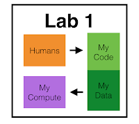
Today, science is produced by the following basic infrastructure. This simplistic picture depicts how humans in a lab interact with the nodes making up the infrastructure. Humans basically use computational resources to analyze data by writing code. The input to these nodes overall is extremely sparse. That is we generally do not have other peoples' data available, we generally cook our own code specifically for our own data, we generally use our own computational resources.


Unit infrastructure for scientific production

This unit is the fundament for academia. Research is carried out by the same infrastructure that is simply replicated across geographies and time. Of course, there could be labs collaborating with each other, of course we could be using an external grid engine to run our tasks, of course we might download a toolbox to run analyses. These are all connections that are not shown in this picture. 

But the emphasis here is that we spent most of our time to reinvent the wheel by
-writing the same piece of code that many people had done it in the past, 
-collecting yet a new dataset instead of generating a new hypothesis compatible with available datasets, 
-buying large computers that could be used by other people
-hiring system administrators that are doing exactly the same work as in another lab
the list is long...


Each lab in this culture becomes a specialized idiosyncratic creature with its own way of doing things. Politically this implies committing in long-term fixed-costs to maintain an academic infrastructure that is short-sighted and benefits mainly to the labs short-term agenda.  Academia mainly benefits from the contributions of labs in the form of publications, which is considered as the unique currency in academic reward system. What is the impact of this system on the society? In the light of current replication crises in science, it is hard to be optimistic.

Infrastructure for academic work. Culture of mine.

This type of infrastructure organization has mainly historical reasons. This model is archaic, and has been a good model for the pre-internet era where people and systems were connected sparsely with each other, where it made sense to travel to a conference and meet other people.

A new way of doing science at the age of cloud-based systems

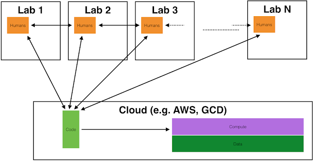
We have to rethink about how to place boxes shown in the previous pictures, how to set novel incentive mechanisms, and how to organize the work flow across scientists and nodes. Let's talk about this simple picture.

A novel infrastructure for academic work. Culture of sharing.

Outsourcing the storage and compute resources to a cloud service (e.g. AWS, GDC or some supranational public cloud service yet to be put in place) are for the benefit of the society in terms of reducing overall costs. 

However the main point here is not about outsourcing storage and compute resources. The real reason for this move is for making datasets accessible to other scientists. And in the long-term this actually means making data to be publicly available to all citizens.

The only thing that is specific to a given lab is the data that is collected there. That's what labs should do: collect data. Most importantly data must to be stored according to strict standardization. That is to each data set, a map has to be associated, that will help people on how to navigate this data set. Furthermore, every dataset should be stored with a minimal code that ensure basic access to data. Also, most often datasets spans multiple modalities. For example, my fMRI datasets are typically bundled together with pupil recordings and heart-beat recordings. We therefore need not only a standardization for storage of specific kind of datasets, but we also need a way to create dataset-bundles that represents an experiment in a flexible manner. A principled way to bundle standardized datasets. Let's call this step 1.

The other thing that labs do is to write code to process their data. To my opinion this is where the biggest challenge is located, namely on finding a system where people can collaborate and create something together. Assuming that the step 1 is solved, the code that is written will also be publicly available. Therefore, code that is written will be directly connected to a dataset type. 

For example, if I am trying to detect peaks in a more or less periodical physiological recording, I will not start looking for literature, find someone's algorithm, implement my version of it. I will simply search for code that is compatible with this type of data, browse among alternative codes, read comments to figure out strengths and weaknesses, consider ratings and incorporate that code to my pipeline.

Basically putting up an analysis will be about creating a pipeline using previously coded nodes or coding new nodes when the analysis has not been previously carried out. When something doesn't work as expected, code needs to be improved via collaboration. Writing good quality code will be one great novel incentive for scientists.

Another challenge is to find a way how to fund this novel system. This is certainly beyond the capacity of a single start-up. This is also beyond the scope of a single lab or institute. I also don't think today's national states are visionary enough to take such moves. To my opinion this could only be established by some tech giants who have the know-how required to solve all these problems.


What is so bad and great in academia?

When you are a scientist working in public service i.e. in academia, a major and constant question you ask will be about identifying deep-rooted problems in academia. While there are actually many bad aspects of academic working conditions, there are also great things about it. This post tries to give an objective pros vs. cons perspective to this question.

I started a list of bad and ugly things that are constantly deteriorating academic life. A list of great things follows below...


  • Pressure for your own future

    Well, no surprise here. If your study fails to find an effect, you are the first one that is affected. You wasted two years of your life and didn't make any progress, your boss lost interest in your project. Depending on the workplace culture you might have absorbed such risks if your project list was diverse enough, but generally the rule is that one person = one project. There is no mechanism currently that absorbs this type of risks. Result: Scientists are pressured to find something, creating overall a bias for falsely finding positive results.

  • Backward publication system


    We publish more or less as Fisher or even Newton. Well we do not really send a post mail but an electronic mail to the editorial office, that is true. But besides that the publication system has not seen a major improvement incorporating anything positive from the era of internet. This model is hackable by short-term benefit seekers and introduces biases in findings. A. Gelman discusses here how changing the publication system by shifting towards an open-post publication reviewing system can create novel incentives for the community.

  • Lack of crowd-based knowledge systems 
    Ratings: ★★★★☆
    412 scientists rated
    this broom with 4.12 stars.
    It is a great broom!

    We scientists read many many papers. But we somehow cannot give any opinions on them. Whereas a person selling a simplest plastic broom could receive harsh comments on Amazon, a person who is writing a bad paper in an high impact journal can easily get away with it. Why can we not simply rate papers online, why can't we create a crowd-sourced reputation system for papers that is fair and transparent in the same time?

  • Culture of mine

    As soon as you are born as a scientist, say when you start you master thesis, you will be assigned to one single project. When you grow up and get your own grant you will do the same, you will assign one project to one person. This makes you live in a bubble and cuts you completely from all sort of sharing tools and mindset that are simply the standard in industry. Unless you dedicate your own time you will never learn great practices of code sharing, writing a code for others, encapsulating your analysis as a toolbox. This is because you work alone for long long periods of time.

  • Pressure for publishing

    Publishing is a key activity in academia. The problem starts as soon as your qualities are judged solely by your publication track record. What about teaching, supervision, peer-reviewing, code sharing, diversity of your publication track record? Nope. At the end of the day, only the impact factor of the journals you published counts. If you started your career in a great lab, but has never published in high-impact journals, you have already started with one leg missing. Combined with the "culture of mine", this opens the way to authorship disputes, that are everywhere.

  • Pressure for short-term thinking 

    Most of the position in academia, are short-term contracts. Great masses are hired by a few professional elites. And these elites are equally free to either plan with you and invest in your career, or to exploit you like a vampire until your contract expires. There is no mechanism that evaluates supervisors in terms of the success of their students.

  • Lack of transparency in evaluation of your work 
    Reviewing papers anonymously.

    It takes on average few years to work on a project and finalize it as a manuscript. The evaluation takes 45 minutes per reviewer that are free too evaluate your manuscript as a crocodile or a sweet hedgehog. Accountability of reviewers is not in the equation, same for inter-reviewer reliability.

  • Predatory seniors

    Academia is a social service, the person who has the title of professor is a civil servant. However, there are no mechanisms that evaluate professors on their performance with this respect. A question like "What did you do to improve scientific practices last year and make the system more efficient ?" is missing.

  • Lack of recognition

    The fact that you can spend a lot of time working in academia and collect lots of expertise and experience, doesn't entitle you with anything significant. As far as I can talk for Germany, you are just an employee, not a hair-dresser, not a pharmacist, you are just an employee. Why don't we have a profession called "scientist"? This is mainly due to the lack of long-term contracts. And I believe very strongly that third party funding is damaging the academic sphere in favor of few strong elites and at the expense talented young scientists.


An article that focuses on only the bad sides cannot be useful for anything. So let's actually talk about what is great in academia.

  • Relative Freedom

    Not being constrained by a final product that needs to do something precise gives us great freedom in the way we work our way through something. As a professor, one reaches the peak of this freedom and can work on any topic at any time. It is just a great thing to be able to start a project any time on any topic without somebody telling "you have not published enough on this topic yet!".

  • Great colleagues

    Working with alike-minded colleagues around you, who are curious and have low thresholds for brainstorming on random topics is a great positive thing. Having a constant hunger for curiosity as a social norm is certainly a positive thing.

  • Publishing a great paper

    Dedicating your efforts on something and walking step by step on that direction is a great source of happiness. And additionally, crowning your final work with a great publication is a priceless reward. It is something you can show your grand (mo/fa)ther and evoke interest on totally random people.

  • Learning doing new things, creativity

    Being able to do things that the overwhelming majority of human population cannot is a great feeling. You have spent all your day doing this weird analysis and it turned out to be completely useless, but well you were unique and used your creativity. To the extent working in academia nourishes this craftsmanship it is an extremely pleasurable occupation.

  • Flexibility in working

    As an academic we are most of the time free on where and when we want to work. You can wake up at 11 and work until midnight or take the opposite approach, it is completely normal to not expect people to conform the regular working class habits.

This is a list I will constantly update and improve. However, this is a great point in time to hear about what people think about the good and bad sides of academia.

SPM Kurs 2018: Batching an SPM preprocessing pipeline.

Untitled

%

% This is a tutorial on scripting an analysis pipeline with SPM in

% Matlab. It follows the SPM course 2018 held in Institute of Systems

% Neuroscience at UKE.

%

% Summary of the pipeline:

% In short, we convert both anatomical and functional dicom images to NifTi

% and merge them into 4D files. Surface representations from anatomical

% images are computed with cat12 toolbox, which also generates deformation

% fields and segmented tissues. Using the segmented tissues we

% skull-strip the anatomical image. Functional images are motion corrected,

% coregistered to skull-striped anatomical image and resliced. The mean EPI

% image that is written during motion correction is segmented and the

% resulting tissue images are used to create a binary mask in native space.

% This mask is used during first-level analysis. The resulting beta images

% are normalized with the deformation fields coming from the

% Surface/Segment routing of the anatomical images and smoothed for second

% level analysis.

%

% Audience;

% People with a basic understanding of programming in Matlab. You need to

% know what is a variable, structure, cell array etc.

%

% SPM version:

% I have used for this spm12 (version: 6685). I suppose any spm12 version

% would be OK to use it. Don't forget to add spm12 to Matlab's path.

%

% Operating System:

% If you are on Windows, for path definitions you will have to either change

% by hand (or with Find and Replace) the / slashes to back slashes \. Or

% alternatively use the filesep function Matlab provides, try

% sprintf('%s',filesep) to see.

%

% Parallelization:

% In many situations, you can take advantage of parallelizing batches

% across multiple CPUs. Currently, this is not optimal: Replicing the for

% loops with parfor loops might or might not always work. If you are

% insisting on this, you may want to compute your matlabbatch{n} variables

% inside a normal for loop, and re-run a second loop using parfor, example:

% parfor k = 1:N;spm_jobman('run', matlabbatch{k});end

%

% Perspective:

% Most of the code that you can read below is simply snippets that are

% taken from our group's analysis and preprocessing pipeline, which I wrote

% with object-oriented programming. If you master batching SPM pipelines

% with the code below, you may find it useful to have a look at my toolbox

% FancyCarp at https://github.com/selimonat/fancycarp

%

% This analysis script assumes that your data is organized as

% project/data/subjectX/runY. For future, it is best to align with the BIDS

% standards.

%

%

Declare Project-level variables that we will use later.

total_subject = 2; %number of participants.

total_run = 3; %number of runs

project_folder = '/home/onat/Desktop/spm-kurs/my_project/data/'; %location of the project data.

dummies_to_delete = 4; %number of dummy scans to delete

TR = 0.99; %in unit of seconds

tpm_dir = '/home/onat/Documents/Code/Matlab/spm12-6685/tpm/'; % path to TPM templates

path_tpm = @(n) sprintf('%s/TPM.nii,%i',tpm_dir,n) % this is an inline function that returns the Nth TPM template

%%%%%%%%%%%%%%%%%%%%%%%%%%%%%%%%%%%%%%%%%%%%%%%%%%%%%%%%%%%%%%%%%%%%%%%%%%%

%%%%%%%%%%%%%%%%% PREPROCESSING OF ANATOMICAL IMAGES%%%%%%%%%%%%%%%%%%%%%%%

%%%%%%%%%%%%%%%%%%%%%%%%%%%%%%%%%%%%%%%%%%%%%%%%%%%%%%%%%%%%%%%%%%%%%%%%%%%

(1.1) DICOM CONVERSION FOR ANATOMICAL IMAGES

%this will convert all dicom files and generate one NifTi file called

%data.nii.

matlabbatch = [];

for subject_number = 1:total_subject

fprintf('Running Subject: %03d\n',subject_number)

%folder where dicom files are located.

destination = sprintf('%ssub%03d/run000/mrt/',project_folder,subject_number)

%find all files in destimation that starts with MR prefix (you may want

%to change MR in line with your needs.

anatomical_files = spm_select('FPListRec',destination,'^MR');

%create batch cell array

matlabbatch{1}.spm.util.import.dicom.data = cellstr(anatomical_files);

matlabbatch{1}.spm.util.import.dicom.root = 'flat';

matlabbatch{1}.spm.util.import.dicom.outdir = {destination};

matlabbatch{1}.spm.util.import.dicom.protfilter = '.*';

matlabbatch{1}.spm.util.import.dicom.convopts.format = 'nii';

matlabbatch{1}.spm.util.import.dicom.convopts.icedims = 0;

%run the batch: will create sTRIO files.

spm_jobman('run', matlabbatch);

%delete dicom files

files = cellstr(anatomical_files);

delete(files{:});

% rename sTRIO... file to data.nii

files = spm_select('FPListRec',destination,'^sTRIO');

movefile(files,regexprep(files,sprintf('%ssTRIO.*$',filesep),sprintf('%sdata.nii',filesep)));%rename it to data.nii

end

(1.2) Runs CAT12 Segment Surface routine.

If you would like to do the conversion via the GUI, you need to first run the CAT12 toolbox from the SPM window, SPM GUI > toolboxes > CAT12 > Preprocessing > Segment Data.

The results of this step are needed for skull stripping.

This is a time consuming part, you may want to parallelize the computation if you have the parallel computing toolbox. I tested this in my computer using parfor, and it worked.

Think thoroughly if you need this step, as it takes considerable time.

Will write to the disk: mri and report folders mri/iy_data.nii mri/p1data.nii mri/p2data.nii mri/wmdata.nii mri_y_data.nii

for subject_number = 1:total_subject

%OR: parfor subject_number = 1:total_subject

fprintf('Running Subject: %03d\n',subject_number)

path_hr = sprintf('%ssub%03d/run000/mrt/data.nii',project_folder,subject_number);

matlabbatch = [];

matlabbatch{1}.spm.tools.cat.estwrite.data = {spm_select('expand',path_hr)};

matlabbatch{1}.spm.tools.cat.estwrite.nproc = 0;

matlabbatch{1}.spm.tools.cat.estwrite.opts.tpm = {sprintf('%sTPM.nii',tpm_dir)};

matlabbatch{1}.spm.tools.cat.estwrite.opts.affreg = 'mni';

matlabbatch{1}.spm.tools.cat.estwrite.extopts.APP = 1;

matlabbatch{1}.spm.tools.cat.estwrite.extopts.LASstr = 0.5;

matlabbatch{1}.spm.tools.cat.estwrite.extopts.gcutstr = 0.5;

matlabbatch{1}.spm.tools.cat.estwrite.extopts.cleanupstr = 0.5;

matlabbatch{1}.spm.tools.cat.estwrite.extopts.darteltpm = {'/home/onat/Documents/Code/Matlab/spm12-6685/toolbox/cat12/templates_1.50mm/Template_1_IXI555_MNI152.nii'};

matlabbatch{1}.spm.tools.cat.estwrite.extopts.vox = 1.5;

matlabbatch{1}.spm.tools.cat.estwrite.output.surface = 1;

matlabbatch{1}.spm.tools.cat.estwrite.output.GM.native = 1;

matlabbatch{1}.spm.tools.cat.estwrite.output.GM.mod = 0;

matlabbatch{1}.spm.tools.cat.estwrite.output.GM.dartel = 0;

matlabbatch{1}.spm.tools.cat.estwrite.output.WM.native = 1;

matlabbatch{1}.spm.tools.cat.estwrite.output.WM.mod = 0;

matlabbatch{1}.spm.tools.cat.estwrite.output.WM.dartel = 0;

matlabbatch{1}.spm.tools.cat.estwrite.output.bias.warped = 1;

matlabbatch{1}.spm.tools.cat.estwrite.output.jacobian.warped= 0;

matlabbatch{1}.spm.tools.cat.estwrite.output.warps = [1 1];

%

spm_jobman('run', matlabbatch);

end

(1.3) Skull Strip anatomical image

Needs results of SegmentSurface, will produce a skullstripped version of hr (ss_data.nii). It will also automatically create a normalized version (w_ss_data.nii).

%path to p1 and p2 images created by SegmentSurface

for subject_number = 1:total_subject

fprintf('Running Subject: %03d\n',subject_number)

path_hr = sprintf('%ssub%03d/run000/mrt/data.nii', project_folder,subject_number);

dir_hr = sprintf('%ssub%03d/run000/mrt/', project_folder,subject_number);

c1 = sprintf('%ssub%03d/run000/mrt/mri/p1data.nii',project_folder,subject_number);

c2 = sprintf('%ssub%03d/run000/mrt/mri/p2data.nii',project_folder,subject_number);

path_skullstrip = sprintf('%ssub%03d/run000/mrt/ss_data.nii', project_folder,subject_number);

deformation_field = sprintf('%ssub%03d/run000/mrt/mri/y_data.nii',project_folder,subject_number);

if exist(c1) && exist(c2) %only strip if C1 and C2 images are present.

matlabbatch = [];

matlabbatch{1}.spm.util.imcalc.input = cellstr(strvcat(path_hr,c1,c2)); %3 volumes that are given as arguments to the calculator

matlabbatch{1}.spm.util.imcalc.output = path_skullstrip;

matlabbatch{1}.spm.util.imcalc.outdir = {dir_hr};

matlabbatch{1}.spm.util.imcalc.expression = 'i1.*((i2+i3)>0.2)'; % operations to be conducted with the 3 images

matlabbatch{1}.spm.util.imcalc.options.dmtx = 0;

matlabbatch{1}.spm.util.imcalc.options.mask = 0;

matlabbatch{1}.spm.util.imcalc.options.interp = 1;

matlabbatch{1}.spm.util.imcalc.options.dtype = 4;

%spm_jobman('run', matlabbatch);

%normalize the skull stripped image as soon as it is

%created.

VolumeNormalize(deformation_field,path_skullstrip);

else

fprintf('Need to run segment first...\n')

end

end

%%%%%%%%%%%%%%%%%%%%%%%%%%%%%%%%%%%%%%%%%%%%%%%%%%%%%%%%%%%%%%%%%%%%%%%%%%%

%%%%%%%%%%%%%%%%% PREPROCESSING OF FUNCTIONAL IMAGES %%%%%%%%%%%%%%%%%%%%%%

%%%%%%%%%%%%%%%%%%%%%%%%%%%%%%%%%%%%%%%%%%%%%%%%%%%%%%%%%%%%%%%%%%%%%%%%%%%

(2.1) DICOM CONVERSION FOR FUNCTIONAL IMAGES and REMOVAL OF DUMMY SCANS

%this will convert all dicom files, delete dummies and generate a 4D NifTi

%file called data.nii.

matlabbatch = [];

for subject_number = 1:total_subject

for run_number = 1:total_run

fprintf('Running Subject: %03d, Run: %03d\n',subject_number,run_number)

% find dicom files in the destination folder

destination = sprintf('%ssub%03d/run%03d/mrt/',project_folder,subject_number,run_number);

% you may need to change ^MR according to your needs.

dicom_files = spm_select('FPListRec',destination,'^MR');

% create the batch.

matlabbatch = [];

matlabbatch{1}.spm.util.import.dicom.data = cellstr(dicom_files);

matlabbatch{1}.spm.util.import.dicom.root = 'flat';

matlabbatch{1}.spm.util.import.dicom.outdir = {destination};

matlabbatch{1}.spm.util.import.dicom.protfilter = '.*';

matlabbatch{1}.spm.util.import.dicom.convopts.format = 'nii';

matlabbatch{1}.spm.util.import.dicom.convopts.icedims = 0;

% run batch: will create fTRIO..nii files.

spm_jobman('run', matlabbatch);

% delete first N dummies.

fprintf('Deleting dummy files\n')

files = spm_select('FPListRec',destination,'^fTRIO');%change fTRIO if your files has a different prefix

files_to_delete = cellstr(files(1:dummies_to_delete,:));

delete(files_to_delete{:});

% merge to 4D

fprintf('Merging fTRIO files into 4D\n')

files = spm_select('FPListRec',destination,'^fTRIO');%change fTRIO if your files has a different prefix

matlabbatch = [];

matlabbatch{1}.spm.util.cat.vols = cellstr(files);

matlabbatch{1}.spm.util.cat.name = 'data.nii';

matlabbatch{1}.spm.util.cat.dtype = 0;

% run batch: will create a file called data.nii

spm_jobman('run', matlabbatch);

% delete all dicom files

fprintf('Deleting dicom images files\n')

dicom_files = cellstr(dicom_files);

delete(dicom_files{:});

% delete all 3D fTRIO files

fprintf('Deleting fTRIOimages files\n')

files = cellstr(files);

delete(files{:});

end

end

%%%%%%%%%%%%%%%%%%%%%%%%%%%%%%%%%%%%%%%%%%%%%%%%%%%%%%%%%%%%%%%%%%%%%%%%%%%

%%%%%%%%%%%%%%%%%%%%%%%%%%%%%%%%%%%%%%%%%%%%%%%%%%%%%%%%%%%%%%%%%%%%%%%%%%%

%%%%%%%%%%%%%%%%%%%%%%%%%%%%%%%%%%%%%%%%%%%%%%%%%%%%%%%%%%%%%%%%%%%%%%%%%%%

(2.2) Realignment and coregistration

We will make a double pass realignment and save only the mean image. This will write rp_data.txt files on the disk for every run. We will than find the best transformation of this mean image to the anatomical one. And finally apply this transformation to all other EPIs and reslice them for further analysis. This will create r_data.nii image.

for subject_index = 1:total_subject

%

fprintf('Running Subject: %03d, Run: %03d\n',subject_index)

% get the EPIs from all runs for this subject

epi_run = [];

c = 0;

for run_index = 1:total_run

c = c +1;

path_epi = sprintf('%ssub%03d/run%03d/mrt/data.nii',project_folder,subject_index,run_index)

files = spm_select('expand',path_epi);

epi_run{c} = cellstr(files);

end

%

mean_epi = sprintf('%ssub%03d/run001/mrt/meandata.nii',project_folder,subject_index);

anatomical = sprintf('%ssub%03d/run000/mrt/data.nii',project_folder,subject_index);

%or this: if you had already an skull striped anatomical image:"

%anatomical = sprintf('%ssub%03d/run000/mrt/ss_data.nii',project_folder,subject_index);

matlabbatch = [];

% double-pass realign EPIs and reslice the mean image only.

matlabbatch{1}.spm.spatial.realign.estwrite.data = epi_run;

matlabbatch{1}.spm.spatial.realign.estwrite.eoptions.quality = 0.9;

matlabbatch{1}.spm.spatial.realign.estwrite.eoptions.sep = 4;

matlabbatch{1}.spm.spatial.realign.estwrite.eoptions.fwhm = 5;

matlabbatch{1}.spm.spatial.realign.estwrite.eoptions.rtm = 1;%double pass

matlabbatch{1}.spm.spatial.realign.estwrite.eoptions.interp = 2;

matlabbatch{1}.spm.spatial.realign.estwrite.eoptions.wrap = [0 0 0];

matlabbatch{1}.spm.spatial.realign.estwrite.eoptions.weight = '';

% we would like to have the mean_image saved for coreg

matlabbatch{1}.spm.spatial.realign.estwrite.roptions.which = [0 1];%write only the mean image for later

matlabbatch{1}.spm.spatial.realign.estwrite.roptions.interp = 4;

matlabbatch{1}.spm.spatial.realign.estwrite.roptions.wrap = [0 0 0];

matlabbatch{1}.spm.spatial.realign.estwrite.roptions.mask = 1;

matlabbatch{1}.spm.spatial.realign.estwrite.roptions.prefix = 'r';

% coregister EPIs to anatomical (only the affine matrix is modified)

% this procedure works best when the skull stripped image is used as

% anatomical reference. You may want to run that batch first below, and

% then adjust above the path to anatomical by adding the ss_ prefix.

matlabbatch{2}.spm.spatial.coreg.estimate.ref = cellstr(anatomical); %the one that is kept immobile

matlabbatch{2}.spm.spatial.coreg.estimate.source = cellstr(mean_epi); %the one that is moved around to best fit

matlabbatch{2}.spm.spatial.coreg.estimate.other = vertcat(epi_run{:}); %all others that are moved around using the best fitting transformation.

matlabbatch{2}.spm.spatial.coreg.estimate.eoptions.cost_fun = 'nmi';

matlabbatch{2}.spm.spatial.coreg.estimate.eoptions.sep = [4 2];

matlabbatch{2}.spm.spatial.coreg.estimate.eoptions.tol = [0.02 0.02 0.02 0.001 0.001 0.001 0.01 0.01 0.01 0.001 0.001 0.001];

matlabbatch{2}.spm.spatial.coreg.estimate.eoptions.fwhm = [7 7];

% write EPIs

matlabbatch{3}.spm.spatial.realign.write.data = vertcat(epi_run{:});

matlabbatch{3}.spm.spatial.realign.write.roptions.which = [2 1];%all images as well as the mean image.

matlabbatch{3}.spm.spatial.realign.write.roptions.interp = 4;

matlabbatch{3}.spm.spatial.realign.write.roptions.wrap = [0 0 0];

matlabbatch{3}.spm.spatial.realign.write.roptions.mask = 1;

matlabbatch{3}.spm.spatial.realign.write.roptions.prefix = 'r';

spm_jobman('run', matlabbatch);

end

to have a look at the motion parameters change to the first run of participant N

a = load('rp_data.txt')

subplot(1,2,1)

plot(a(:,1:3))

subplot(1,2,2)

plot(a(:,4:6))

(2.3) Skull Strip mean-EPI image but first segment mean EPI

Same as what we did with the anatomical image. The skull stripped mean image will be handy to use it as a mask for the first-level analysis. Will make it faster. However to compute a skull strip mean EPI we need the results of segmentation. We will not run this time CAT12's segmentation, but instead spm's default segmentation.

(2.3A) Runs the new segment of SPM12 on the mean EPI image.

Will write to the disk: meandata_seg8.mat iy_meandata.nii c{1-5}meandata.nii y_meandata.nii

for subject_index = 1:total_subject

path_meanepi = sprintf('%ssub%03d/run001/mrt/meandata.nii',project_folder,subject_index);

matlabbatch = [];

matlabbatch{1}.spm.spatial.preproc.channel.vols = cellstr(path_meanepi);

matlabbatch{1}.spm.spatial.preproc.channel.biasreg = 0.001;

matlabbatch{1}.spm.spatial.preproc.channel.biasfwhm = 60;

matlabbatch{1}.spm.spatial.preproc.channel.write = [0 0];

matlabbatch{1}.spm.spatial.preproc.tissue(1).tpm = {path_tpm(1)};

matlabbatch{1}.spm.spatial.preproc.tissue(1).ngaus = 1;

matlabbatch{1}.spm.spatial.preproc.tissue(1).native = [1 0];

matlabbatch{1}.spm.spatial.preproc.tissue(1).warped = [0 0];

matlabbatch{1}.spm.spatial.preproc.tissue(2).tpm = {path_tpm(2)};

matlabbatch{1}.spm.spatial.preproc.tissue(2).ngaus = 1;

matlabbatch{1}.spm.spatial.preproc.tissue(2).native = [1 0];

matlabbatch{1}.spm.spatial.preproc.tissue(2).warped = [0 0];

matlabbatch{1}.spm.spatial.preproc.tissue(3).tpm = {path_tpm(3)};

matlabbatch{1}.spm.spatial.preproc.tissue(3).ngaus = 2;

matlabbatch{1}.spm.spatial.preproc.tissue(3).native = [1 0];

matlabbatch{1}.spm.spatial.preproc.tissue(3).warped = [0 0];

matlabbatch{1}.spm.spatial.preproc.tissue(4).tpm = {path_tpm(4)};

matlabbatch{1}.spm.spatial.preproc.tissue(4).ngaus = 3;

matlabbatch{1}.spm.spatial.preproc.tissue(4).native = [1 0];

matlabbatch{1}.spm.spatial.preproc.tissue(4).warped = [0 0];

matlabbatch{1}.spm.spatial.preproc.tissue(5).tpm = {path_tpm(5)};

matlabbatch{1}.spm.spatial.preproc.tissue(5).ngaus = 4;

matlabbatch{1}.spm.spatial.preproc.tissue(5).native = [1 0];

matlabbatch{1}.spm.spatial.preproc.tissue(5).warped = [0 0];

matlabbatch{1}.spm.spatial.preproc.tissue(6).tpm = {path_tpm(6)};

matlabbatch{1}.spm.spatial.preproc.tissue(6).ngaus = 2;

matlabbatch{1}.spm.spatial.preproc.tissue(6).native = [0 0];

matlabbatch{1}.spm.spatial.preproc.tissue(6).warped = [0 0];

matlabbatch{1}.spm.spatial.preproc.warp.mrf = 1;

matlabbatch{1}.spm.spatial.preproc.warp.cleanup = 1;

matlabbatch{1}.spm.spatial.preproc.warp.reg = [0 0.001 0.5 0.05 0.2];

matlabbatch{1}.spm.spatial.preproc.warp.affreg = 'mni';

matlabbatch{1}.spm.spatial.preproc.warp.fwhm = 0;

matlabbatch{1}.spm.spatial.preproc.warp.samp = 3;

matlabbatch{1}.spm.spatial.preproc.warp.write = [1 1];

spm_jobman('run', matlabbatch);

end

(2.3B) skullstrip the mean EPIs, creating a mask in native space

for subject_index = 1:total_subject

path_meanepi_segmented = ''

for n = 1:3

path_meanepi_segmented = strvcat(path_meanepi_segmented, sprintf('%ssub%03d/run001/mrt/c%dmeandata.nii',project_folder,subject_index,n));

end

Vout = sprintf('%ssub%03d/run001/mrt/ss_meandata.nii',project_folder,subject_index); %output volume that will be written to disk

spm_imcalc(path_meanepi_segmented,Vout,'(i1+i2+i3)>0')

end

%check out the results using Mango, you must see a nice binary volume in native space

%that we can use for masking first level analysis.

(2.3) First-level analysis

This section relies on the data that is stored in runYYY/design/modelXX

folder. Each modelXX folder contains one specific model. Organizing

models in separate folders will help you encapsulate results

in one folder specific for one analysis. This is because spm will write

the results of an analysis using modelXX in a folder names spm/modelXX/

What is contained in the modelXX is folder is data.mat file that

contains information about stimulus onsets. When you load data.mat to

the workspace, this spawns a structure array called cond. The fields

names of the cond are organized exactly the same way SPM expects onset

information. Therefore, this Matlab structure can be directly fed into

the matlabbatch variable without further massaging.

What is important also is that the motion parameters that we computed

above will be inserted as nuisance covariates.

This batch will write the SPM.mat file together with beta images.

model_num = 1;

path_skullstrip_meanepi = sprintf('%ssub%03d/run001/mrt/ss_meandata.nii',project_folder,subject_index);

for subject_number = 1:total_subject

spm_dir = sprintf('%ssub%03d/run001/spm/model%02d/',project_folder,subject_number,model_num);

path_spm = sprintf('%ssub%03d/run001/spm/model%02d/SPM.mat',project_folder,subject_number,model_num);

deformation_field = sprintf('%ssub%03d/run000/mrt/mri/y_data.nii',project_folder,subject_number);

matlabbatch = [];

matlabbatch{1}.spm.stats.fmri_spec.dir = {spm_dir};

matlabbatch{1}.spm.stats.fmri_spec.timing.units = 'scans';

matlabbatch{1}.spm.stats.fmri_spec.timing.RT = TR;

matlabbatch{1}.spm.stats.fmri_spec.timing.fmri_t = 16;

matlabbatch{1}.spm.stats.fmri_spec.timing.fmri_t0 = 1;

for session = 1%:total_run

%location of EPIs

path_epi = sprintf('%ssub%03d/run%03d/mrt/rdata.nii',project_folder,subject_number,session);

matlabbatch{1}.spm.stats.fmri_spec.sess(session).scans = cellstr(spm_select('expand',path_epi));%use always the realigned data.

%location of onsets

path_model = sprintf('%ssub%03d/run%03d/design/model%02d/data.mat',project_folder,subject_number,session,model_num);

dummy = load(path_model);

matlabbatch{1}.spm.stats.fmri_spec.sess(session).cond = struct('name', {}, 'onset', {}, 'duration', {}, 'tmod', {}, 'pmod', {});

matlabbatch{1}.spm.stats.fmri_spec.sess(session).cond = dummy.cond;

%load nuissance parameters

path_param_motion = sprintf('%ssub%03d/run%03d/mrt/rp_data.txt',project_folder,subject_number,session);

nuis = load(path_param_motion);

nuis = zscore([nuis [zeros(1,size(nuis,2));diff(nuis)] nuis.^2 [zeros(1,size(nuis,2));diff(nuis)].^2 ]);

for nNuis = 1:size(nuis,2)

matlabbatch{1}.spm.stats.fmri_spec.sess(session).regress(nNuis).val = nuis(:,nNuis);

matlabbatch{1}.spm.stats.fmri_spec.sess(session).regress(nNuis).name = mat2str(nNuis);

end

%

matlabbatch{1}.spm.stats.fmri_spec.sess(session).multi = {''};

matlabbatch{1}.spm.stats.fmri_spec.sess(session).multi_reg = {''};

matlabbatch{1}.spm.stats.fmri_spec.sess(session).hpf = 128;

end

matlabbatch{1}.spm.stats.fmri_spec.fact = struct('name', {}, 'levels', {});

matlabbatch{1}.spm.stats.fmri_spec.bases.hrf.derivs = [0 0];%we have [0 0], [ 1 0] or [ 1 1] for 1, 2, or 3 regressors.

matlabbatch{1}.spm.stats.fmri_spec.volt = 1;

matlabbatch{1}.spm.stats.fmri_spec.global = 'None';

matlabbatch{1}.spm.stats.fmri_spec.mthresh = -Inf;%

matlabbatch{1}.spm.stats.fmri_spec.mask = {path_skullstrip_meanepi}; %use the native mask we computed above.

matlabbatch{1}.spm.stats.fmri_spec.cvi = 'none';

spm_jobman('run', matlabbatch);%create SPM file first

%estimation

matlabbatch = [];

matlabbatch{1}.spm.stats.fmri_est.spmmat = {path_spm};

matlabbatch{1}.spm.stats.fmri_est.method.Classical = 1;

spm_jobman('run', matlabbatch);

% As you must have remarked, we did not yet smoothened the EPI images,

% which is slightly odd with typical processing pipelines.

% The idea is that smoothing is a linear operator. And linear operators are

% commutative, whether you do first A and then B, is the same as B and then

% A if A and B operations are linear. Given that modelling and smoothing

% are linear operations, we can first fit a model and then to the smoothing

% and normalization for the second-level. This saves tremendous amounts of

% disk space.

% Have a look at the following thread in the SPM maillist:

%https://www.jiscmail.ac.uk/cgi-bin/webadmin?A2=ind00&L=spm&P=R30456&1=spm&9=A&I=-3&J=on&X=3C2B8009325E6AC405&Y=sonat%40uke.de&d=No+Match%3BMatch%3BMatches&z=4

% normalize, apply deformation field to beta images.

total_beta = 10;% Bulk of beta images are about nuissance images, which we are not interesting.

% we will smooth and normalize only the

% first TOTAL_BETA images. This will

% different depending on your model.

beta_weights = '';

for n = 1:total_beta

beta_weights = strvcat(beta_weights , sprintf('%sbeta_%04d.nii',spm_dir,n));

end

VolumeNormalize(deformation_field,beta_weights)

% and smooth.

beta_weights = '';

for n = 1:total_beta

beta_weights = strvcat(beta_weights , sprintf('%sw_beta_%04d.nii',spm_dir,n));

end

VolumeSmooth(beta_weights,8);

end

(2.4) Second-level analysis using ANOVA

2nd level analysis only makes sense with smoothened and normalized images, thus we seek for beta images with a prefix s_w_.

The result of this analysis are stored in project_path/spm/modelXX in the form of beta images. You can then select the SPM.mat file from SPM GUI and make statistical analyses using the contrast GUI.

total_beta = 10;

model_num = 1;

spm_dir = sprintf('%sseconlevel/model%02d/',project_folder,model_num);

matlabbatch = [];

for beta_index = 1:total_beta

%collect the beta image for a given condition for all participants

beta_images = '';

for subject_index = 1:total_subject

beta_images = strvcat(beta_images,sprintf('%ssub%03d/run001/spm/model%02d/s_w_beta_%04d.nii',project_folder,subject_number,model_num,beta_index));

end

%and store it in an ANOVA cell.

matlabbatch{1}.spm.stats.factorial_design.des.anova.icell(beta_index).scans = cellstr(beta_images );

end

%

matlabbatch{1}.spm.stats.factorial_design.dir = cellstr(spm_dir);

matlabbatch{1}.spm.stats.factorial_design.des.anova.dept = 0;

matlabbatch{1}.spm.stats.factorial_design.des.anova.variance = 1;

matlabbatch{1}.spm.stats.factorial_design.des.anova.gmsca = 0;

matlabbatch{1}.spm.stats.factorial_design.des.anova.ancova = 0;

matlabbatch{1}.spm.stats.factorial_design.cov = struct('c', {}, 'cname', {}, 'iCFI', {}, 'iCC', {});

matlabbatch{1}.spm.stats.factorial_design.multi_cov = struct('files', {}, 'iCFI', {}, 'iCC', {});

matlabbatch{1}.spm.stats.factorial_design.masking.tm.tm_none = 1;

matlabbatch{1}.spm.stats.factorial_design.masking.im = 1;

matlabbatch{1}.spm.stats.factorial_design.masking.em = {''};

matlabbatch{1}.spm.stats.factorial_design.globalc.g_omit = 1;

matlabbatch{1}.spm.stats.factorial_design.globalm.gmsca.gmsca_no = 1;

matlabbatch{1}.spm.stats.factorial_design.globalm.glonorm = 1;

%

matlabbatch{2}.spm.stats.fmri_est.spmmat = {[spm_dir '/SPM.mat']};

matlabbatch{2}.spm.stats.fmri_est.method.Classical = 1;

%

spm_jobman('run', matlabbatch);